astrohack

Cassegrain Ray Tracing tutorial¶

This tutorial was created to clarify the usage of the Cassegrain ray tracing tools. These tools were created as a proof of concept of using ray tracing to simulate phase effects caused by small optical misalignments in holography apertures. On previous holography experiments, e.g. VLA holographies, these phase effects were fitted out of apertures by using a phase model derived by Ruze (1969), this model assumes that the path length perturbations are small and hence only the first-degree terms are used. This type of “phase fitting” is very powerful, however it relies on the misalignments being small and on the fact of the VLA using a modified version of the Cassegrain optical design. For the case of the ngVLA this is no longer the case and both reflectors used shaped optics, and thus it is very hard to estimate phase effects on the aperture analytically. Hence the need for a Ray tracing model of the ngVLA.

The toy model presented here is a proof of concept, that can be checked against the phase fitting algorithm already present in astrohack.

[1]:

import os

try:
    import astrohack

    print("AstroHACK version", astrohack.__version__, "already installed.")
except ImportError as e:
    print(e)
    print("Installing AstroHACK")

    os.system("pip install astrohack")

    import astrohack

    print("astrohack version", astrohack.__version__, " installed.")

AstroHACK version 1.0.1 already installed.

Setting up¶

In this step we create the variables containing the names of the files to be created, as well as the folder to contain the plots and ray tracing file.

[2]:

# Setting up file names and a folder to contain data
datafolder = "vla-rt-data"
os.makedirs(datafolder, exist_ok=True)
vla_rt_filename = datafolder + "/VLA-rt.zarr"
plot_base_names = datafolder + "/vla-rt"

Initiate Telescope parameters¶

To run the ray tracing pipeline, we need a set of parameters to describe the optics of the telescope to be simulated. The expected format for these parameters is a dictionary, the function below creates such a dictionary. Below we fill the parameters of this function with the appropriate values for the VLA, according to EVLA memo 211.

[3]:

from astrohack import create_ray_tracing_telescope_parameter_dict

vla_pars = create_ray_tracing_telescope_parameter_dict(
    primary_diameter=25,  # 25 meters for the VLA
    secondary_diameter=2.5146,  # VLA's Secondary diameter
    focal_length=9.0,  # VLA's focal length
    z_intercept=3.140,  # Distance between the z intercept of the secondary and the point between the 2 foci
    foci_half_distance=3.662,  # Half distance between the 2 foci
    inner_radius=2.0,  # Inner blockage
    horn_diameter=0.2,  # Horn diameter
    length_unit="m",  # Unit for the dimensions given
)

print()
for key, item in vla_pars.items():
    print(f"{key:20s} = {item}")
print()

[2026-03-19 15:39:18,813]     INFO   astrohack:  Module path: /export/home/arya/work/Holography-1022/astrohack/src/astrohack

primary_diameter     = 25.0
secondary_diameter   = 2.5146
focal_length         = 9.0
z_intercept          = 3.14
foci_half_distance   = 3.662
inner_radius         = 2.0
horn_diameter        = 0.2
horn_position        = [0, 0, 1.6760000000000002]
horn_orientation     = [0, 0, 1]

Plotting phases and other interesting products¶

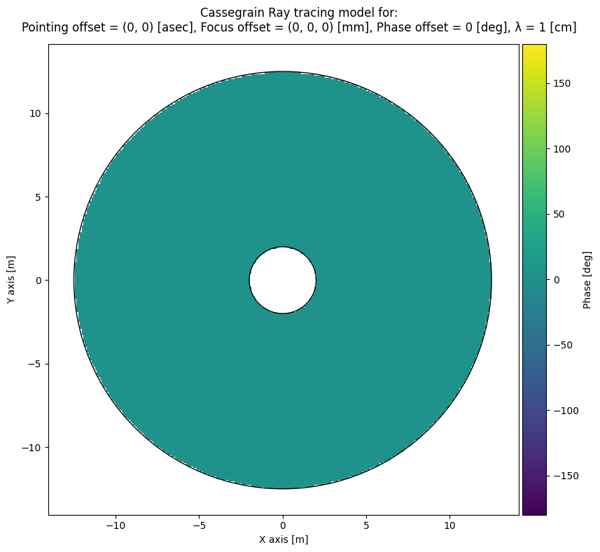
Since the data variables in the rt_xds have to be gridded in order to be properly viewed a convenience function was created to allow easy access to its data variables. The variables that can be accessed this way are the ones that have points as their first dimension, excepting image_indexes as it only contains the information needed to regrid the points to 2D images.

[6]:

from astrohack import plot_2d_maps_from_rt_xds

plot_2d_maps_from_rt_xds(
    rt_xds_filename=vla_rt_filename,  # Name of the input XDS file with RT results
    keys=["phase", "total_path"],  # Keys to be plotted
    rootname=plot_base_names,  # Base name for plot files
    phase_unit="deg",  # Unit for phase plots
    length_unit="m",  # Unit for other available keys
    colormap="viridis",  # Colormap to be used in plots
    display=True,  # Display plots below
    dpi=300,  # Resolution for the png plots
)

[2026-03-19 15:39:21,769]     INFO   astrohack:  Module path: /export/home/arya/work/Holography-1022/astrohack/src/astrohack

../_images/tutorials_cassegrain_ray_tracing_tutorial_13_1.png

../_images/tutorials_cassegrain_ray_tracing_tutorial_13_2.png

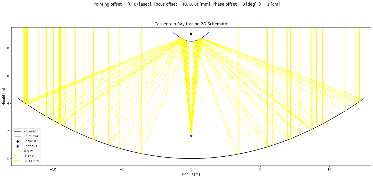
Radial projection plot¶

Another interesting visualization is the projection of the rays as seen from a cross section across the middle of the primary dish. This allows us to track the path of rays from the sky and into the horn. The user is encouraged to play with the ray tracing parameters and check when rays simply stop being detected at the horn. It is also interesting to make this plot with nrays=0 to obtain a simplified schematic of the telescope’s optical design.

[7]:

from astrohack import plot_radial_projection_from_rt_xds

plot_radial_projection_from_rt_xds(
    rt_xds_filename=vla_rt_filename,  # RT XDS filename
    plot_filename=plot_base_names
    + "rz.png",  # Name of the file to be saved to disk with the plot
    nrays=50,  # No rays plotted here
    display=True,  # Display plot below
    dpi=300,  # Resolution for the png plot
)

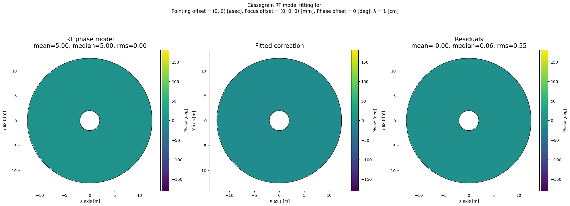
[2026-03-19 15:39:23,452]     INFO   astrohack:  Module path: /export/home/arya/work/Holography-1022/astrohack/src/astrohack

../_images/tutorials_cassegrain_ray_tracing_tutorial_15_1.png

Comparison to Astrohack’s VLA phase fitting¶

Last but not least, we have a check against the phase fitting mechanism present in astrohack.holog. For this analysis is important to understand that some phase effects are in fact degenerated with each other. A Z offset of the secondary reflector creates a ringing effect on the phases but also a large phase offset, which makes the phase offset mildly degenerate with the focus offset, making it difficult to isolate one effect from the other. Similarly, X & Y displacements of the secondary are degenerate with pointing offsets. Hence if the user wants to check if a pointing offset is recovered by the phase fitting algorithm, they should set fit_xy_secondary_offset to False, and vice versa. Unfortunately, it is not possible to do the same with the focus offset as it not possible to turn off the phase offset in the phase fitting algorithm. It is also important to bear in mind that the phase fitting algorithm is not capable of fitting phase offsets larger than ~1 arc minute, or secondary offsets larger than ~3 mm.

[8]:

%%time
from astrohack import apply_holog_phase_fitting_to_rt_xds

apply_holog_phase_fitting_to_rt_xds(
    rt_xds_filename=vla_rt_filename,  # RT XDS filename
    phase_plot_filename=plot_base_names
    + "vs-fit.png",  # Name of the file to be saved to disk with the phase comparison plot
    fit_pointing_offset=True,  # Fit pointing offsets
    fit_xy_secondary_offset=True,  # Fit secondary offsets in the X&Y directions
    fit_focus_offset=True,  # Fit Z offsets of the secondary
    phase_unit="deg",  # Unit for phases in plots
    colormap="viridis",  # Colormap for phase plots
    display=True,  # Display plot below
    dpi=300,  # Resolution for the png plot
)

[2026-03-19 15:39:24,558]     INFO   astrohack:  Module path: /export/home/arya/work/Holography-1022/astrohack/src/astrohack
Comparison between input and fitted values
+----------------+-------------+-----------+-------------------------+------+
|   Parameter    |    Value    | Reference |        Difference       | unit |
+----------------+-------------+-----------+-------------------------+------+
|  Phase offset  | 0.061 ± 0.0 |    0.0    |   0.061374206952080984  | deg  |
| X point offset |  0.0 ± 0.0  |     0     |  2.027335002312594e-13  | asec |
| Y point offset |  0.0 ± 0.0  |     0     |  1.8728984559192682e-13 | asec |
| X focus offset |  0.0 ± 0.0  |     0     |  -1.509267669881906e-14 |  mm  |
| Y focus offset |  0.0 ± 0.0  |     0     | -1.5123879580191193e-14 |  mm  |
| Z focus offset | 0.056 ± 0.0 |     0     |   0.05645696565210622   |  mm  |
+----------------+-------------+-----------+-------------------------+------+

../_images/tutorials_cassegrain_ray_tracing_tutorial_17_1.png

CPU times: user 4.12 s, sys: 76.7 ms, total: 4.2 s
Wall time: 4.22 s